
1. 데이터셋 불러오기
[Empty Module #1] load_dataset
- csv 파일로 구성된 2D 이미지 데이터를 numpy 형태로 가져오기
# -------------------------------------
# [Empty Module #1] 학습데이터, 평가데이터 불러오기
# -------------------------------------


# -------------------------------------
# load_dataset(path, split): <= 코드를 추가하여 학습데이터를 불러오는 코드를 완성하세요
# -------------------------------------
# 목적: 학습데이터 불러오기
# 입력인자: path - 데이터 경로, split - train인지 test인지 여부
# 출력인자: split="TRAIN"일 경우 : train_images - 학습데이터(2D img), 학습라벨(ex. Faces, airplanes,,,,)
#          split="TEST"일 경우 : test_images - 평가데이터(2D img)
# -------------------------------------


def load_dataset(path, split):

    if split == 'TRAIN':
        train_images = []
        train_labels = []
        classes = os.listdir(path)

        for cls_ in tqdm(classes):
            cls_images = os.listdir(os.path.join(path, cls_))

            for cls_img in cls_images:
                # ------------------------------------------------------------
                # 구현 가이드라인  (1)
                # ------------------------------------------------------------
                # 경로의 이미지를 읽어와서 numpy 형태로 변경 후
                # 1D 데이터를 2D 형태인 RGB 데이터(256,256,3)로 변환하고
                # uint64로 제공된 데이터를 astype를 사용하여 uint8로 변경
                # ------------------------------------------------------------
                # 구현 가이드라인을 참고하여 아래쪽에 코드를 추가하라
                image = pd.read_csv(os.path.join(path, cls_, cls_img))
                image = np.array(image).reshape(256,256,3)
                image = image.astype('uint8')

                train_images.append(image)
                train_labels.append(cls_)
                # ------------------------------------------------------------
        return np.array(train_images), np.array(train_labels) # (3060, 256, 256, 3), (3060)


    elif split == 'TEST':
        img_name = sorted(os.listdir(path))
        test_images = []
        for img in tqdm(img_name):
            # ------------------------------------------------------------
            # 구현 가이드라인
            # ------------------------------------------------------------
            # 경로의 이미지를 읽어와서 numpy 형태로 변경 후
            # 1D 데이터를 2D 형태인 RGB 데이터(256,256,3)로 변환하고
            # uint64로 제공된 데이터를 astype를 사용하여 uint8로 변경
            # ------------------------------------------------------------
            # 구현 가이드라인을 참고하여 아래쪽에 코드를 추가하라
            image = pd.read_csv(os.path.join(path, img))
            image = np.array(image).reshape(256,256,3)
            image = image.astype('uint8')

            test_images.append(image)
            # ------------------------------------------------------------
        return np.array(test_images) # (1712, 256, 256, 3)
#경로 설정
train_path = 'train_csv_v2'
test_path = 'test_csv_v2'
label_path = 'Label2Names.csv'#train, test에 대해 load_dataset 함수 실행
train_images, train_labels_ = load_dataset(train_path, 'TRAIN')
test_images = load_dataset(test_path, 'TEST')
label_to_index
- 클래스 명을 범주형 라벨로 변환하는 함수
- (예) "crocodile_head" -> 30
- "BACKGRAOUND_Google"은 Label2Names.csv 안에 없으며, 102로 매핑해서 사용 할 예정
def label_to_index(train_labels_, label_path):

    label_name = pd.read_csv(label_path, header = None)
    label_map = dict()

    for i in range(len(label_name)):
        label_map[label_name[1][i]] = i+1

    label_map['BACKGROUND_Google'] = 102

    train_labels = [label_map[train_labels_[i]] for i in range(len(train_labels_))]

    return train_labels
#분류기 학습에 사용할 label 정보 미리 추출하기

train_labels = label_to_index(train_labels_, label_path)
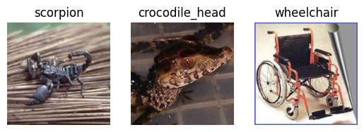
+ numpy 형태로 불러온 Caltech 101 데이터셋 그림으로 살펴보기
(index를 바꿔가면서 데이터셋의 구성을 살펴보세요)
from matplotlib import pyplot as plt

fig = plt.figure()
rows = 1
cols = 3

img1 = train_images[7]
img1 = cv2.cvtColor(img1, cv2.COLOR_RGB2BGR)

img2 = train_images[77]
img2 = cv2.cvtColor(img2, cv2.COLOR_RGB2BGR)

img3 = train_images[777]
img3 = cv2.cvtColor(img3, cv2.COLOR_RGB2BGR)

ax1 = fig.add_subplot(rows, cols, 1)
ax1.imshow(img1)
ax1.set_title(train_labels_[7])
ax1.axis("off")

ax2 = fig.add_subplot(rows, cols, 2)
ax2.imshow(img2)
ax2.set_title(train_labels_[77])
ax2.axis("off")

ax2 = fig.add_subplot(rows, cols, 3)
ax2.imshow(img3)
ax2.set_title(train_labels_[777])
ax2.axis("off")

plt.show()
2. 특징점, 기술자 추출하기
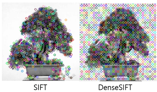
[Empty Module #2] extract_descriptor
- 아래 모듈 'else' 블럭의 일반 SIFT 코드를 참고해서, 'if isDense is True' 블럭 채우기
- SIFT의 detect 함수와 compute 함수를 활용한다.
- SIFT의 detect 함수는 특징점 위치를 추출하는 함수이고, compute 함수는 특징점 위치에서 주변 정보를 기술하는 기술자를 추출하는 함수이다.
- (힌트 : DenseSIFT의 경우는 이미지 내 모든 영역에 Dense하게 특징점이 존재한다고 가정하는 방법론이므로 step_size = 8 로 설정하여 이미지 내에 특징점을 먼저 설정한 후 sift compute를 진행하기)
- (라이브러리 라이선스 이슈 때문에 cv2.xfeatures2d.SIFT_create() 말고 cv2.SIFT_create() 사용할 것)
- documentation 참고
isDense = True
# True : DenseSIFT,  False : 일반 SIFT
# -------------------------------------
# [Empty Module #2] 특징점 추출하기
# -------------------------------------
# -------------------------------------
# extract_descriptor(img, isDense = False):
# -------------------------------------
# 목적: 이미지 내에서 특징점(feature point)을 추출(detect)하고 기술(describe)하기
# 입력인자: img - numpy형태 이미지, isDense - DenseSIFT인지 아닌지 여부
# 출력인자: des - 이미지의 특징점에서 기술된 기술자(descriptor)
# -------------------------------------
def extract_descriptor(img, isDense = False):
sift = cv2.SIFT_create()
if isDense is True: # DenseSIFT 추출
step_size = 8
# ------------------------------------------------------------
# 구현 가이드라인
# ------------------------------------------------------------
# cv2.KeyPoint 함수를 사용해 step_size=8 만큼의 dense한 특징점 설정
# -(kp는 cv2.Keypoint 객체들을 담는 list로 세팅)
# -(256x256의 이미지 사이즈에서 step_size=8일 경우 32x32=1024개의 특징점 생성. 따라서 len(kp)=1024)
# cv2.cvtColor 함수를 사용해 이미지를 gray 형태로 변형 (SIFT 추출을 위해)
# 미리 설정한 특징점으로 부터 SIFT 기술자(descriptor) 추출
# ------------------------------------------------------------
# 구현 가이드라인을 참고하여 아래쪽에 코드를 추가하라
kp = [cv2.KeyPoint(x, y, step_size) for y in range(0, img.shape[0], step_size)
for x in range(0, img.shape[1], step_size)]
gray = cv2.cvtColor(img, cv2.COLOR_BGR2GRAY)
_, des = sift.compute(gray, kp)
# ------------------------------------------------------------
else: # 일반 SIFT 추출
gray = cv2.cvtColor(img, cv2.COLOR_BGR2GRAY)
_, des = sift.detectAndCompute(gray, None)
return des# Codebook 생성을 위해 학습 이미지 전체에서 기술자 추출하기
train_descriptors = [extract_descriptor(train_img, isDense = isDense) for train_img in tqdm(train_images)]
train_descriptors = np.array(train_descriptors, dtype="object")
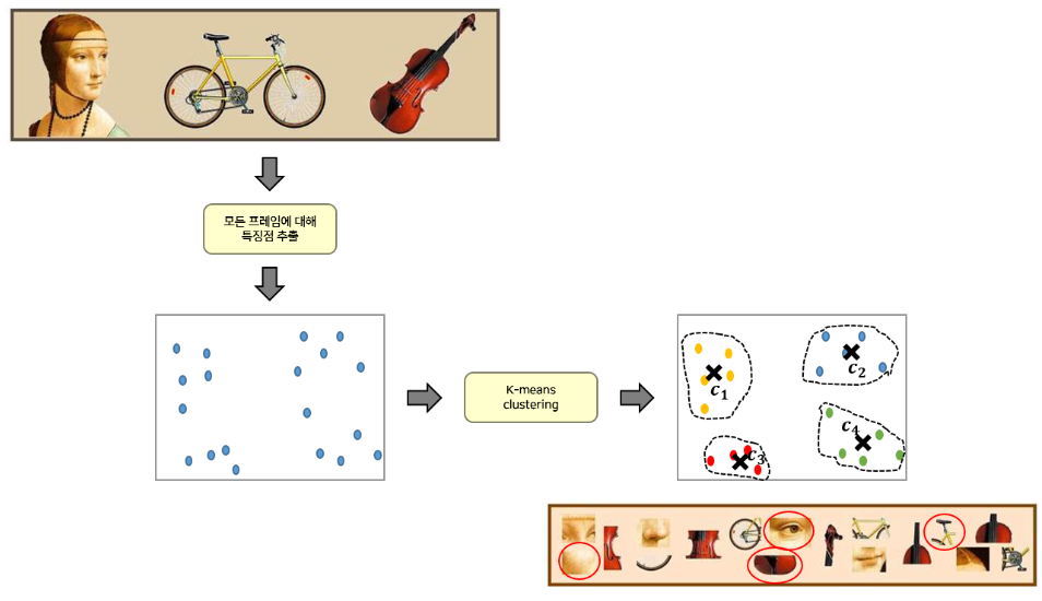
3. Codebook 생성
- 추출한 SIFT (or DenseSIFT)의 기술자(descriptor)를 사용해서 Codebook 생성
- 위에서 구한 train_descriptors는 모든 학습 이미지에서 특징점(visual word)를 구한 것이다.
- 수 많은 특징점(visual word) 중 K-Means clustering을 통해 대표가 되는 특징점(codeword)들을 선정하고 이들을 묶어서 codebook을 만들어야 한다.
- 특징점(codeword)의 수는 baseline에서 모두 200으로 세팅
n_codeword = 200def build_codebook_GPU(X,voc_size, isDense = True):
if isDense:
feature=np.array(X).reshape(-1,128).astype('float32')
else:
feature = np.empty((0,128))
for x in tqdm(X):
feature = np.append(feature, x, axis=0)
feature = feature.reshape(-1,128).astype('float32')
d=feature.shape[1]
k=voc_size
clus = faiss.Clustering(d, k)
clus.niter = 300
clus.seed =8
clus.max_points_per_centroid = 10000000
ngpu=1
res = [faiss.StandardGpuResources() for i in tqdm(range(ngpu))]
flat_config = []
for i in tqdm(range(ngpu)):
cfg = faiss.GpuIndexFlatConfig()
cfg.useFloat16 = False
cfg.device = i
flat_config.append(cfg)
if ngpu == 1:
index = faiss.GpuIndexFlatL2(res[0], d, flat_config[0])
clus.train(feature, index)
centroids = faiss.vector_float_to_array(clus.centroids)
centroids=centroids.reshape(k, d)
return centroids # codeword들이 모인 codebook 구하기
codebook = build_codebook_GPU(train_descriptors, n_codeword, isDense)
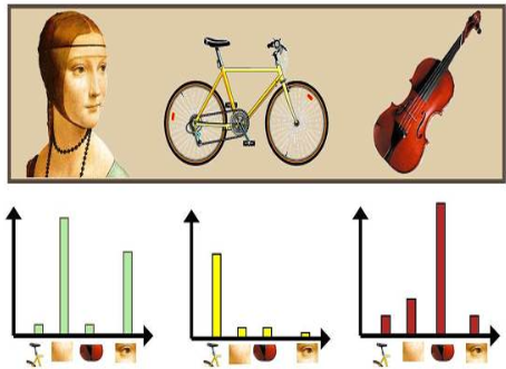
4. BOVW, VLAD vector 생성
[Empty Module #3] BOVW
- 생성해둔 codebook(kmeans clustrer center) 와 특징점(visual word)을 비교하여 histogram을 구하는 작업 진행
- scipy.cluster.vq를 사용해 각 특징점(visual word)과 유사한 codebook의 Index를 반환 받아 사용
- (메뉴얼 참고)
- vq를 이용해 얻은 Index를 np.histogram 을 사용해 histogram을 구한다
- np.histogram 사용 시 bin의 range를 (0, n_codeword+1)로 설정
- (메뉴얼 참고)
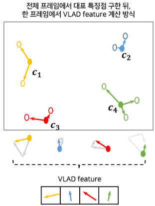
[Empty Module #4] VLAD
- BOVW에서는 각 특징점(visual word)와 유사한 codebook의 Index를 사용했다면,
- VLAD 에서는 각 특징점(visual word)을 codebook내 대표 특징점(codeword) 중 가장 유사한 것과 벡터 차이를 계산한 후, 동일한 대표 특징점(codeword)에 할당된 특징점(visual word)의 벡터 차이 값을 모두 더해주는 방식으로 VLAD feature를 기술
#BOVW 기술자와 VLAD 기술자 중 어떤 것을 사용할지 선정

args_desc = "VLAD"  # "BOVW" or "VLAD"
# -------------------------------------
# [Empty Module #3] BOVW 알고리즘
# -------------------------------------
# -------------------------------------
# BOVW(descriptor, codebook):
# -------------------------------------
# 목적: Histogram (즉, 빈도수)를 계산하기 위한 함수 (BOVW 기술자를 계산하기 위한 함수)
# 입력인자: descriptor - 한 이미지에서 추출된 기술자(descriptor)들의 모음 ([1024,128] --> DenseSIFT의 경우 1024)
# codebook - 학습데이터 전체를 대표하는 codeword들의 모음 ([200,128])
# 출력인자: hist - feature의 codebook 빈도수(즉 histogram)을 flatten한 Matrix
# -------------------------------------
from scipy.cluster.vq import vq
def BOVW(descriptor, codebook):
# ------------------------------------------------------------
# 구현 가이드라인
# ------------------------------------------------------------
# 1) scipy.cluster.vq 를 사용해 각 특징점(visual word)과 가장 유사한 codebook의 Index를 반환
# 2) 구한 Index들 histogram을 np.histogram 을 사용해 histogram을 구한다
# 2-Tip) np.histogram 사용시 bin의 range를 (0, n_codeword+1)로 설정
# ------------------------------------------------------------
# 구현 가이드라인을 참고하여 아래쪽에 코드를 추가하라
words, _ = vq(descriptor, codebook)
hist, _ = np.histogram(words, bins=np.arange(codebook.shape[0] + 1))
# ------------------------------------------------------------
return hist -------------------------------------
# [Empty Module #4] VLAD 알고리즘
# -------------------------------------
# -------------------------------------
# VLAD(descriptor, codebook):
# -------------------------------------
# 목적: VLAD 기술자를 계산하기 위한 함수
# 입력인자: descriptor - 한 이미지에서 추출된 기술자(descriptor)들의 모음 ([1024,128] --> DenseSIFT의 경우 1024)
# codebook - 학습데이터 전체를 대표하는 codeword들의 모음 ([200,128])
# 출력인자: V - 계산한 VLAD 기술자
# -------------------------------------
def VLAD(descriptor, codebook):
#VLAD 기술자를 담기 위한 변수
V = np.zeros([codebook.shape[0], descriptor.shape[1]])
# ------------------------------------------------------------
# 구현 가이드라인
# ------------------------------------------------------------
# 1) scipy.cluster.vq 를 사용해 각 특징점(visual word)과 가장 유사한 codebook의 Index를 반환
# 2) 동일한 대표 특징점(codeword)으로 할당된 특징점(visual word)들의 벡터 합 계산해 V[i]에 저장
# (한 이미지에서 얻게 되는 VLAD 기술자인 V의 shape은 (n_codeword,128))
# ------------------------------------------------------------
# 구현 가이드라인을 참고하여 아래쪽에 코드를 추가하라
words, _ = vq(descriptor, codebook)
for i in range(codebook.shape[0]):
if np.sum(words == i) > 0:
V[i] = np.sum(descriptor[words == i] - codebook[i], axis=0)
# ------------------------------------------------------------
# 후처리 과정
V = V.flatten()
V = np.sign(V)*np.sqrt(np.abs(V))
if np.sqrt(np.dot(V,V))!=0:
V = V/np.sqrt(np.dot(V,V))
return V
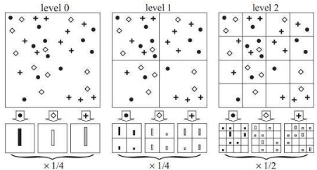
+ <Spatial Pyramid Matching 기법>
- Spatial Pyramid Matching 방법에서는 여기에 추가적으로 이미지를 점진적으로 세분(level 1에서는 2x2로 분할, level 2에서는 4x4로 분할, ...)해 가면서 각각의 분할 영역마다 별도로 히스토그램을 구한 후,
- 이들 히스토그램들을 전부 모아서 일종의 피라미드(pyramid)를 형성
- (level=0일 경우 Spatial Pyramid Matching을 적용하지 않고, 영상 전체에 대해서 한번만 기술자를 추출한다.)
[Empty Module #5] cut_image
- Spatial Pyramid Matching 기법 적용을 위해 입력 이미지를 자르는(cut) 함수
- 입력 이미지를 입력 level에 맞게 잘라서 새로운 리스트(cutted_img)에 담은 뒤 return 하는 역할
- 만약 level=1일 경우 함수에서 반환하는 리스트(cutted_img)의 길이는 4가 된다.
#Spatial Pyramid Matching 의 사용 여부 결정하기
#[0]으로 세팅할 경우 전통적인 기법들 처럼 level 0만 사용하게 되고,
#[0,1,2]로 세팅할 경우 level 0,1,2 모두를 더해 예측에 사용

pyramid_levels = [0, 1] # [0] or [0,1], [0,1,2] 로 세팅 가능
# -------------------------------------
# [Empty Module #5] cut_image 함수
# -------------------------------------
# -------------------------------------
# cut_image(img, level):
# -------------------------------------
# 목적: Spatial Pyramid Matching을 위해 입력 이미지를 level에 맞게 자르는 함수
# 입력인자: img - 자르고자 하는 입력 이미지
# level - 자를 level 선정 (overview 그림 참고)
# 출력인자: cutted_img - 자른 이미지를 담은 리스트
# -------------------------------------
def cut_image(img, level):
if level == 0: # level이 0이기 때문에 Spatial Pyramid Matching을 적용하지 않는다. 따라서 입력 img 그대로 return
return [img]
else: # Spatial Pyramid Matching을 적용하는 경우
h_end, w_end, _ = img.shape #입력 이미지의 높이와 너비
cutted_img = [] #자른 이미지를 담을 리스트
w_start = 0
h_start = 0
w = w_end // (2**level)
h = h_end // (2**level)
# ------------------------------------------------------------
# 구현 가이드라인
# ------------------------------------------------------------
# 입력 level에 맞게 입력 이미지를 잘라서 cutted_img에 append 해주기
# 반복문 돌때마다 w_start와 h_start 를 새롭게 갱신해주기
# ------------------------------------------------------------
# 구현 가이드라인을 참고하여 아래쪽에 코드를 추가하라
for i in range((2 ** level)): # 레벨 1에서는 원본이미지를 4등분(2x2), 레벨2에서는 원본이미지에서 16등분(4x4)함
for j in range(2 ** level):
w_start = j * w
h_start = i * h
cutted_img.append(img[h_start:h_start + h, w_start:w_start + w])
# ------------------------------------------------------------
return cutted_img# 학습, 테스트 이미지를 세팅한 pyramid_levels 에 대해 자르고(cut),
# 자른 이미지에 대해 각각 BOVW 또는 VLAD 구하기
train_vec = []
for level in pyramid_levels:
pyramid_histogram = []
for train_img in tqdm(train_images):
pyramid_hist = []
cut_imgs = cut_image(train_img, level)
for cut_img in cut_imgs:
desc_cut = extract_descriptor(cut_img, isDense = isDense)
if desc_cut is not None:
if args_desc == "BOVW":
hist_cut = BOVW(desc_cut, codebook)
elif args_desc == "VLAD":
hist_cut = VLAD(desc_cut, codebook)
pyramid_hist.extend(hist_cut)
if len(pyramid_hist) !=0:
pyramid_histogram.append(np.array(pyramid_hist))
else:
# 일반 SIFT (Dense X)에서 SIFT 검출이 안된 이미지의 경우 에러 방지를 위해 임의로 0 채우기
pyramid_histogram.append(np.zeros(200).astype('int64'))
train_vec.append(np.array(pyramid_histogram))
test_vec = []
for level in pyramid_levels:
pyramid_histogram = []
for test_img in tqdm(test_images):
pyramid_hist = []
cut_imgs = cut_image(test_img, level)
for cut_img in cut_imgs:
desc_cut = extract_descriptor(cut_img, isDense = isDense)
if desc_cut is not None:
if args_desc == "BOVW":
hist_cut = BOVW(desc_cut, codebook)
elif args_desc == "VLAD":
hist_cut = VLAD(desc_cut, codebook)
pyramid_hist.extend(hist_cut)
if len(pyramid_hist) !=0:
pyramid_histogram.append(np.array(pyramid_hist))
else:
# 일반 SIFT (Dense X)에서 SIFT 검출이 안된 이미지의 경우 에러 방지를 위해 임의로 0 채우기
pyramid_histogram.append(np.zeros(200).astype('int64'))
test_vec.append(np.array(pyramid_histogram))# PCA 차원 축소 적용
from sklearn.decomposition import PCA
def apply_pca(train_vec, test_vec, n_components=100):
pca = PCA(n_components=n_components)
all_train_vec = np.vstack(train_vec)
all_test_vec = np.vstack(test_vec)
pca.fit(all_train_vec)
train_vec_pca = [pca.transform(vec) for vec in train_vec]
test_vec_pca = [pca.transform(vec) for vec in test_vec]
return train_vec_pca, test_vec_pca
train_vec, test_vec = apply_pca(train_vec, test_vec, n_components=100)5. SVM : 분류기 학습
[Empty Module #6] SVM
- 앞서 구한 정보를 사용하여 SVM 분류기 학습
- 베이스라인 파라미터는 default 유지. <svm.SVC()>

train_vectors = np.array([])

for vec in train_vec:
    if train_vectors.size == 0:
        train_vectors = vec
    else:
        train_vectors = np.hstack((train_vectors, vec))


test_vectors = np.array([])

for vec in test_vec:
    if test_vectors.size == 0:
        test_vectors = vec
    else:
        test_vectors = np.hstack((test_vectors, vec))
# -------------------------------------
# [Empty Module #6] SVM 분류기 학습
# -------------------------------------
def SVM(train_vectors, train_labels, test_vectors):
# ------------------------------------------------------------
# 구현 가이드라인
# ------------------------------------------------------------
# 모든 baseline성능은 clf = svm.SVC(random_state=seed) 로 예측한 성능임
# 분류기로 예측한 최종 예측값을 반환하는 함수
# ------------------------------------------------------------
# 구현 가이드라인을 참고하여 아래쪽에 코드를 추가하라
clf = svm.SVC(random_state=seed)
clf.fit(train_vectors, train_labels)
predict = clf.predict(test_vectors)
# ------------------------------------------------------------
return predictpredict = SVM(train_vectors, train_labels, test_vectors)
<성능 향상을 위한 팁>
- VLAD 기술자의 경우 벡터들의 합에 대한 정보를 가지게 됩니다. 이때 최종 벡터 합들의 크기 값을 균등하게 scaling 해 보면 어떨까요?
- 결국 이미지를 표현하는 기술자들은 codebook의 codeword와의 계산을 통해 구해집니다. codeword의 역할에 대해 잘 생각해보시길 바랍니다.
- Spatial Pyramid Matching에서 level 값을 더 다채롭게 조정해보면 어떨까요?
- PCA 차원 축소를 통해 메모리 부족 이슈가 있는 VLAD 에서도 Spatial Pyramid Matching을 사용해보면 어떨까요?
'Computer Science > Machine Learning' 카테고리의 다른 글
| 앙상블-배깅 (구현) (0) | 2024.06.11 |
|---|---|
| Decision Tree (구현) (0) | 2024.06.11 |
| Linear Classification (구현) (0) | 2024.06.11 |
| Linear Regression (구현) (0) | 2024.06.11 |
| Feature Extract : CV [2D 이미지 데이터를 활용한 이미지 분류] (6) (1) | 2024.06.10 |