0. Abstract
확산 확률 모델과 랑게빈 역학과의 노이즈 제거 점수 매칭 사이의 새로운 연결에 따라 설계된 가중 가변 바운드에 대한 훈련을 통해 최상의 결과를 얻을 수 있으며, 우리 모델은 자동 회귀 디코딩의 일반화로 해석할 수 있는 점진적 손실 압축 해제 방식을 자연스럽게 인정한다.
1. Introduction

DDPM은 주어진 이미지에 time에 따른 상수의 파라미터를 갖는 작은 가우시안 노이즈를 time에 대해 더해나가는데, image가 destroy하게 되면 결국 noise의 형태로 남는다. (normal distribution을 따르는) 이런 상황에서 normal distribution에 대한 noise가 주어졌을 때, image를 어떻게 복원할 것인가에 대한 문제로, 주어진 noise에서 완전히 이미지를 복구한다면 image generation하는 것이 된다.
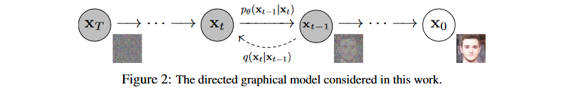
이 논문에서는 diffusion probabilistic models의 과정을 보여준다. diffusion model은 유한한 시간 뒤에 이미지를 생성하는 variational inference(변현 추론)을 통해 훈련된 Markov chain을 parameterized한 형태이다. Markov Chain은 이전의 샘플링이 현재 샘플링에 영향을 미치는 $p(x∣x)$ 형식을 의미한다. 그래서 이 diffusion model에서의 한 방향에 대해서는 주어진 이미지에 작은 gaussian noise를 점진적으로 계속 더해서 완전히 image가 destroy 되게하는 과정을 의미한다.
- Variational inference(변분추론): 사후확률(posterior) 분포 $p(z∣x)$를 다루기 쉬운 확률분포 $q(z)$로 근사(approximation)하는 것
- Parameterize: 하나의 표현식에 대해 다른 parameter를 사용하여 다시 표현하는 과정. 이 과정에서 보통 parameter의 개수를 표현 식의 차수보다 적은 수로 선택(ex. 3차 표현식 → 2개 parameter 사용)하므로, 낮은 차수로의 mapping 함수(ex. 3D --> 2D)가 생성
- Markov chain: 어떤 상태에서 다른 상태로 넘어갈 때, 바로 전 단계의 상태에만 영향을 받는 확률 과정
2. Background
Diffusion model에서 중요한 개념은 'Stochastic Process'로, 시간에 따라 확률이 달라지는 time-dependent variables를 통해 이루어진다.
(1) Forward(Diffusion) Process : $q(x_t|x_{t-1})$

Markov chain으로 data에 노이즈를 추가하는 과정으로, Gaussian noise를 추가할 때 variance schedule $\beta _1,,,\beta_T$로 scaling을 한 후 더해준다.
- $\beta _t = 1$이면 mean인 $\sqrt{1-\beta_t}x_{t-1} = 0$이 되어 이전 정보를 갖지 못하고 noise가 증가한다.
- $\sqrt{1-\beta_t}$로 scaling하는 이유는 variance가 발산하는 것을 막기 위해서이다.
- $q(x_1|x_0)$ : $x_0$에 noise를 추가해 $x_1$을 만드는 과정
- $x_T$는 완전히 destroy된 noise 상태 ~ $N(x_T;0,I)$
(2) Backward(Reverse) Process : $p(x_{t-1}|x_t)$

Forward process가 가우시안이면 reverse process도 가우시안으로 쓰면 된다라는 증명이 있기 때문에, backward process로 가우시안 노이즈를 사용한다.
$x_t$로 평균 $\mu _\theta$과 분산 ${\sum}_{\theta}$을 예측해야 한다.
- Hierarachical VAE에서의 decoding 과정과 비슷하다.
- 과 분산 ${\sum}_{\theta}$는 학습 가능한 parameter이다.
(3) Loss Function : $L$
모델의 목적은 주어진 noise에 대해서 점진적으로 걷어내는 것이다. 그 방법은 위의 backward process인 $p$로 해결할 것이다. $x_t$로 $x_t-1$을 예측할 수 있게 된다면, $x_0$ 또한 예측할 수 있게 된다. 이때 과정은 mean과 variance를 파라미터로 갖는 gaussian 분포에 대해 이루어진다. Generative model이기 때문에, log likelihood를 최대화하기 위해서 negative log likelihood를 최소화하는 방향으로 진행한다.

위 수식을 ELBO(Evidence of Lower BOund)로 우항과 같이 정리하면, Variational bound는 우항과 같이 나오고 이를 풀어내면
ELBO의 역할은 우리가 관찰한 P(z|x)가 다루기 힘든 분포를 이루고 있을 때 이를 조금 더 다루기 쉬운 분포인 Q(x)로 대신 표현하려 하는 과정에서 두 분포 (P(z|x)와 Q(x))의 차이 (KL Divergence)를 최소화 하기 위해 사용된다.

와 같은 결과가 나온다.
- : Regularization term으로 $를 학습시킴
- : Reconstruction term으로 매 단계에서 noise를 지움
- : Reconstruction term으로 최종 단계에서 image를 생성
특이한 점은 forward process의 posterior와 reverse process를 KL Divergence를 통해 직접 비교한다는 것이다. 생각해보면 forward process에 대한 정보를 가지고 있고 forward process의 posterior는 reverse process와 연관이 깊은 형태이기 때문에 tractable하다.
Posterior(사후확률)
사후확률은 베이즈 정리로 근사할 수 있다.
$P(x|z) = \frac{P(z|x) * P(x)}{P(z)}$
$P(x|z) \propto P(z|x) * P(x)$
$P(posterior) \propto likelihood \times P(prior)$
- likelihood : $p(z|x)$, 어떤 모델에서 해당 데이터(관측값)이 나올 확률
- 사전확률(prior probability) : $p(x)$, 관측자가 관측을 하기 전에 시스템 또는 모델에 대해 가지고 있는 선험적 확률. 예를 들어, 남여의 구성비를 나타내는 p(남자), p(여자) 등이 사전확률에 해당한다.
- 사후확률(posterior probability) : $p(x|z)$, 사건이 발생한 후(관측이 진행된 후) 그 사건이 특정 모델에서 발생했을 확률
3. Diffusion models and denoising autoencoders
DDPM에서는 inductive bias(학습 모델이 지금까지 만나보지 못했던 상황에서 정확한 예측을 하기 위해 사용하는 추가적인 가정, 즉 우리가 풀려는 문제에 대한 정보를 모델에 적용하는 것)를 늘려 모델을 더 stable하고 성능도 개선할 수 있었음.
(1) Forward process and $L_T$
- Foward process의 분산 $\beta_t$를 고정한다($10^{-4}$ ~ $0.02$로 linear하게 image에 가까울수록 noise를 적게 주는 방식으로 설정)
- $q$에는 학습 가능한 파라미터가 없기 때문에, $L_T$는 0이 되어 무시해도 된다.
(2) Reverse process and $L_{1:T-1}$
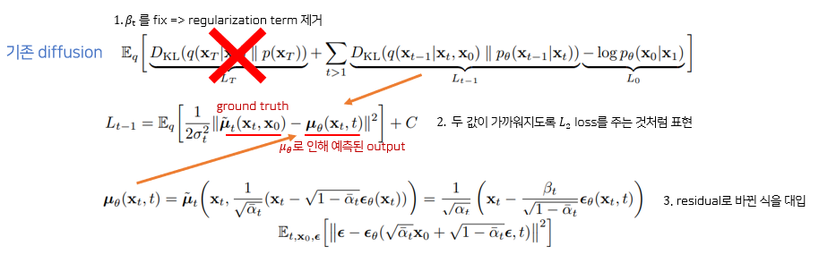
$L_{t-1} = D_{KL}(q(x_{t-1}|x_t,x_0)\left| \right|p_\theta (x_{t-1}|x_t))$
- $q(x_{t-1}|x_t,x_0) = N(x_{t-1};\widetilde{\mu}(x_t,x_0),\widetilde{\beta _t}I)$
- $p_\theta (x_{t-1}|x_t) = N(x_{t-1};\mu _\theta (x_t,t),\sum{_\theta}(x_t,t))$
$L_{1:T-1}$
Foward progress posterior를 예측하는 loss이다. $x_{t-1}$에서 noise를 더해 $x_t$를 만들었을 때, 그 과정을 복원 $p(x_{t-1}|x_t)$하는 과정을 학습한다.
$\sum {_\theta }$
$\beta$를 상수로 가정했기 때문에, $\beta$에 영향을 받는 $p(x_{t-1}|x_t)$의 variance를 학습시키지 않아도 된다. 그렇기 때문에 variance term을 제거한다.
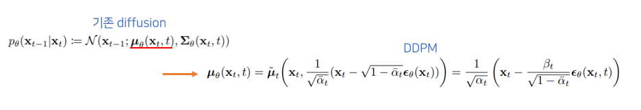
$\mu _\theta $
$\mu _\theta$ 를 바로 구하지 않고, residual $\epsilon _\theta$ 만 구해 정확도를 높였다.
(3) Data scaling, reverse process decoder, and $L_0$
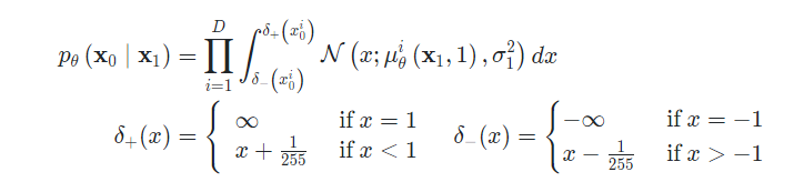
[0, 255]의 image를 [-1,1] 사이로 linearly mapping. Sampling 마지막 단계에는 noise를 추가하지 않음.
$L_0$은 두 normal distribution 사이의 KL divergence를 나타냄
- $D$ : Data Dimensionality
- $i$ : 좌표
(4) Simplified training objective
최종 loss는 위와 같이 나타난다. Ground truth - estimated output간 MSE loss를 줄이는 과정이 denoising과 비슷해 DDPM이라는 이름이 붙음.
Simplified objective을 통해 diffusion process를 학습하면 매우 작은 $t$ 에서뿐만 아니라 큰 $t$에 대해서도 network 학습이 가능하기 때문에 매우 효과적이다.
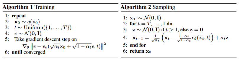
Algorithm 1 : Training
- Noise를 더해가는 과정, network($\epsilon _\theta , p_\theta$)가 $t$ step에서 noise($\epsilon$)가 얼마나 더해졌는지 학습
- 학습 시에는 특정 step의 이미지가 얼마나 gaussian noise가 추가되었는지를 예측하도록 학습됨
- (Code) 랜덤 noise와 시간 단계 t로 noise가 추가된 이미지를 얻고, 해당 이미지를 보고 모델이 노이즈를 예측
def p_losses(self, x_start, t, noise = None):
        b, c, h, w = x_start.shape
        noise = default(noise, lambda: torch.randn_like(x_start))

        # noise sample

        x = self.q_sample(x_start = x_start, t = t, noise = noise)

        # if doing self-conditioning, 50% of the time, predict x_start from current set of times
        # and condition with unet with that
        # this technique will slow down training by 25%, but seems to lower FID significantly

        x_self_cond = None
        if self.self_condition and random() < 0.5:
            with torch.no_grad():
                x_self_cond = self.model_predictions(x, t).pred_x_start
                x_self_cond.detach_()

        # predict and take gradient step

        model_out = self.model(x, t, x_self_cond)

        if self.objective == 'pred_noise':
            target = noise
        elif self.objective == 'pred_x0':
            target = x_start
        elif self.objective == 'pred_v':
            v = self.predict_v(x_start, t, noise)
            target = v
        else:
            raise ValueError(f'unknown objective {self.objective}')

        loss = self.loss_fn(model_out, target, reduction = 'none')
        loss = reduce(loss, 'b ... -> b (...)', 'mean')

        loss = loss * extract(self.loss_weight, t, loss.shape)
        return loss.mean()
Algorithm 2 : Sampling
- Network를 학습하고 나면, gaussian noise에서 시작해서 순차적으로 denoising하는 것이 가능 (by parameterized markov chain)
- (Code) Noise 제거 후 소량의 noise를 다시 추가하고 있음
@torch.no_grad()
def p_sample(self, x, t: int, x_self_cond = None):
    b, *_, device = *x.shape, x.device
    batched_times = torch.full((b,), t, device = x.device, dtype = torch.long)
    model_mean, _, model_log_variance, x_start = self.p_mean_variance(x = x, t = batched_times, x_self_cond = x_self_cond, clip_denoised = True)
    noise = torch.randn_like(x) if t > 0 else 0. # no noise if t == 0
    pred_img = model_mean + (0.5 * model_log_variance).exp() * noise
    return pred_img, x_start
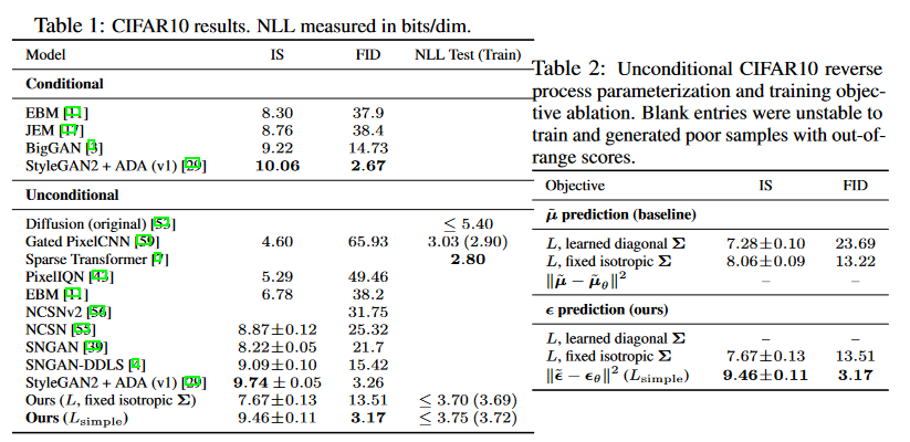
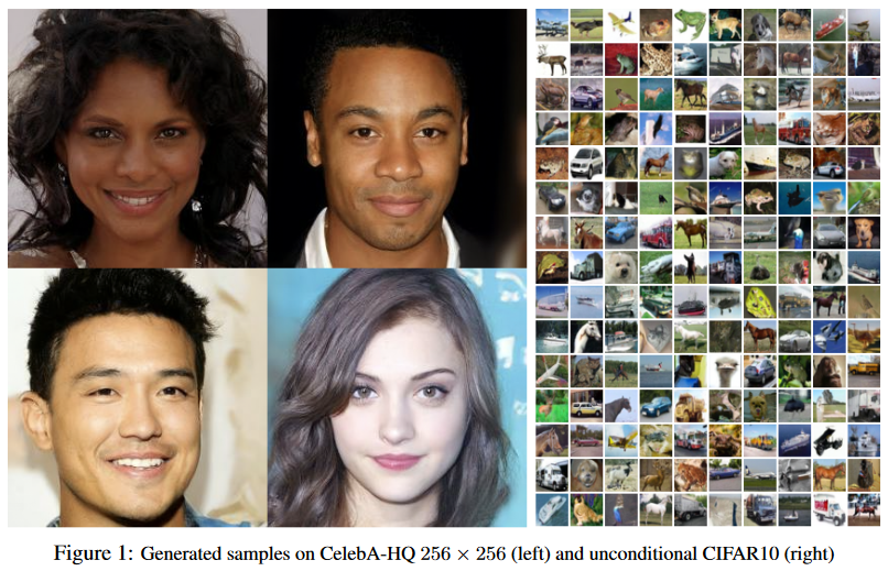
4. Experiments
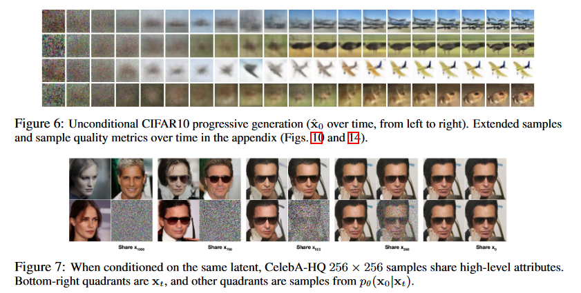
DDPM의 핵심은 reverse process의 $L_{t-1}$(noise)을 이미지의 형태로 다시 정의한 것에 있다. 이렇게 forward process와 reverse process를 정의하여 generative 모델을 구성하고, 이들로부터 사진 데이터를 만들어보면, 좋은 퀄리티의 사진을 만들어 냄을 알 수 있다.