CNN(합성곱 신경망) ② [MNIST]

# 랜덤시드 고정하기
import random
import torch
import numpy as np
import os

seed = 42
random.seed(seed)
np.random.seed(seed)
torch.manual_seed(seed)
if torch.cuda.is_available():
    torch.cuda.manual_seed(seed)
    torch.cuda.manual_seed_all(seed)
torch.backends.cudnn.benchmark = False
torch.backends.cudnn.deterministic = True

 

1. Load MNIST Dataset

# MNIST 데이터 셋 불러오기
from torchvision.datasets import MNIST

download_root = './MNIST_DATASET'

train_dataset = MNIST(download_root, train=True, download=True) # train 데이터
test_dataset = MNIST(download_root, train=False, download=True) # test 데이터

 

2. Visualize the First Six Training Images

# 시각화를 위해 필요한 라이브러리 import
import matplotlib.pyplot as plt
%matplotlib inline
import matplotlib.cm as cm
import numpy as np

# 불러온 데이터 셋 중 처음 6개 이미지에 대한 시각화
fig = plt.figure(figsize=(20,20))
for i in range(6):
    ax = fig.add_subplot(1, 6, i+1, xticks=[], yticks=[])
    ax.imshow(train_dataset[i][0], cmap='gray')
    ax.set_title(str(train_dataset[i][1]))

 

3. View an Image in More Detail

# 이미지의 픽셀값이 어떻게 구성되어 있는지 시각화하는 함수
def visualize_input(img, ax):
    ax.imshow(img, cmap='gray')
    img = np.array(img)
    width, height = img.shape

    #배경색에 따라 글자색을 바꿔주기 위한 임계값 지정
    thresh = img.max()/2.5
    print(img.max())
    print(thresh)

    # 시각화
    for x in range(width):
        for y in range(height):
            ax.annotate(str(round(img[x][y],2)), xy=(y,x),
                        horizontalalignment='center',
                        verticalalignment='center',
                        color='white' if img[x][y]<thresh else 'black')

# figsize에는 inch단위 parameter
fig = plt.figure(figsize = (12,12))

# 111은 1행, 1열, 1번째 plot의미. (1,1,1)과 동일
ax = fig.add_subplot(111)

# 이미지 시각화 
visualize_input(train_dataset[5][0], ax)

 

4. Preprocess input images: Rescale the Images by Dividing Every Pixel in Every Image by 255

# rescale to have values within 0 - 1 range [0,255] --> [0,1]
# pytorch에서는 torchvision.transforms.ToTensor를 이용하여 [0, 1]까지의 정규화와 torch.FloatTensor형으로 형변환을 함께 진행함.

from torchvision import transforms

mnist_transform = transforms.Compose([
    transforms.ToTensor(), 
    ])

train_dataset = MNIST(download_root, transform=mnist_transform, train=True, download=True) # train 데이터
test_dataset = MNIST(download_root, transform=mnist_transform, train=False, download=True) # test 데이터

print(len(train_dataset), 'train samples')  # 60000 train samples
print(len(test_dataset), 'test samples')    # 10000 test samples

 

5. Preprocess the labels: Encode Categorical Integer Labels Using a One-Hot Scheme

# torch.nn.CrossEntropyLoss에 one-hot encoding 내장

import torch
import torch.nn.functional as F

num_classes = 10 
# print first ten (integer-valued) training labels
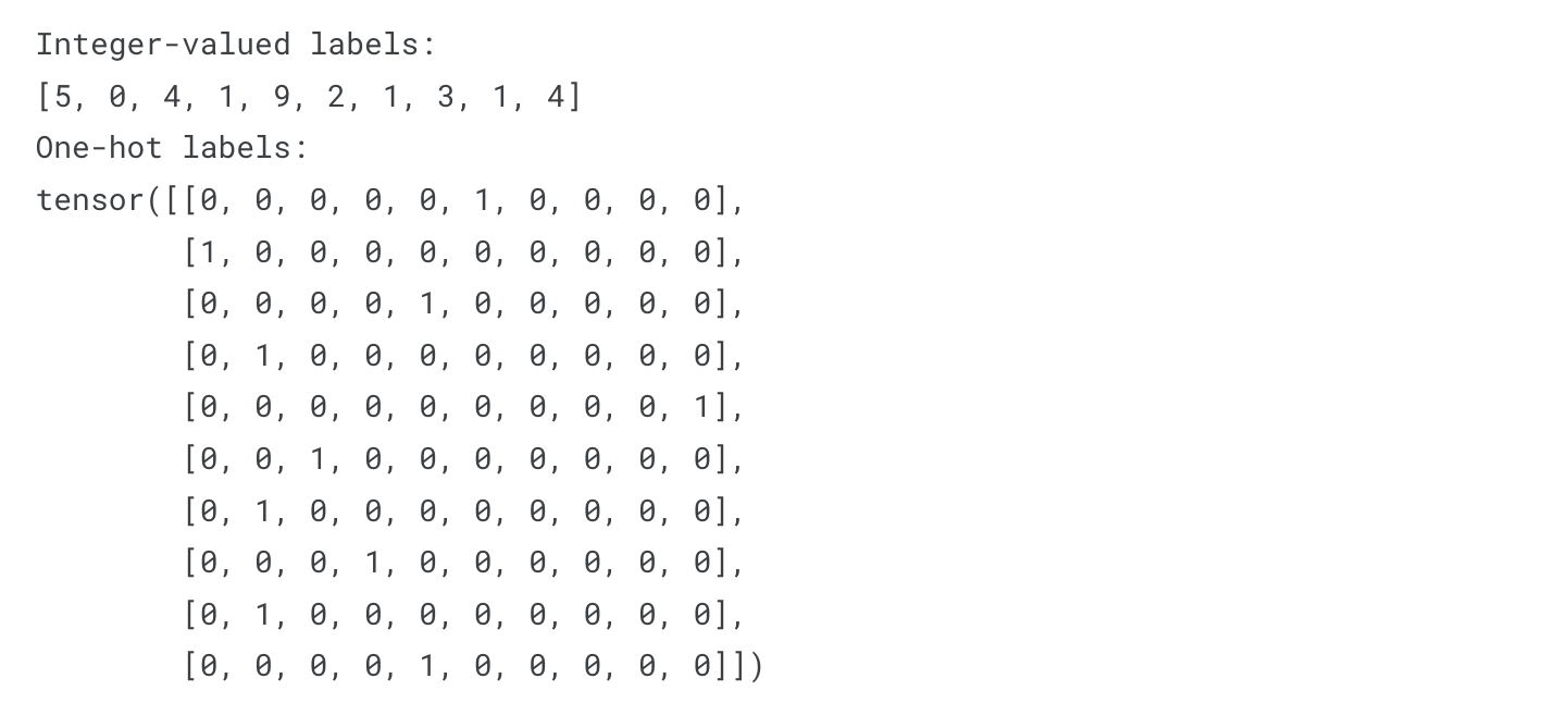
print('Integer-valued labels:')
y_train_list = [train_dataset[i][1] for i in range(10) ]
print(y_train_list)

# one-hot encode the labels
# convert class vectors to binary class matrices
y_train = F.one_hot(torch.tensor(y_train_list), num_classes)

# print first ten (one-hot) training labels
print('One-hot labels:')
print(y_train[:10])

 

7. Define the Model Architecture

%pip install torchsummary ## model을 요약하기 위해 torchsummary 설치
from torchsummary import summary as summary_## 모델 정보를 확인하기 위해 torchsummary 함수 import

## 모델의 형태를 출력하기 위한 함수 
def summary_model(model,input_shape=(1, 28, 28)):
    model = model.cuda()
    summary_(model, input_shape) ## (model, (input shape))

 

# CNN 모델 구조 정의
from torch.nn import Sequential
from torch.nn import Conv2d, MaxPool2d, Flatten, Linear, Dropout, ReLU, ZeroPad2d, Softmax

## nn.Sequential 함수는 네트워크를 인스턴스화하는 동시에, 원하는 신경망에 연산 순서를 인수로 전달함.
model = Sequential(
            Conv2d(1,32,kernel_size=3,padding='same'),  ## 참고: Conv2d(in_channel, out_channel, kernerl_size, padding, bias)
            ReLU(),
            MaxPool2d(kernel_size=2),    
            Conv2d(32,64,kernel_size=3,padding='same'),
            ReLU(),
            MaxPool2d(kernel_size=2),   
            Flatten(),
            Linear(3136,64),
            ReLU(),
            Linear(64,10),
            Softmax(dim=1)
        ).cuda()

print(model)
summary_model(model)  # 모델 요약하기

 

8. Train

# 모델 학습하기
import time

## train, test 데이터셋의 로더
## 배치사이즈와 불러오는 데이터를 섞을지 결정할 수 있다
trainloader = torch.utils.data.DataLoader(train_dataset, batch_size=32,shuffle=True) ## train 로더
testloader = torch.utils.data.DataLoader(test_dataset, batch_size=1,shuffle=False)## test 로더

# 파라미터 설정
total_epoch = 12
best_loss = 100 ## loss를 기준으로 best_checkpoint를 저장하기 위해 100으로 설정하였음.

learning_rate = 0.001 

optimizer = torch.optim.RMSprop(model.parameters(),lr = learning_rate, alpha=0.9, eps=1e-07) ## RMSprop을 최적화 함수로 이용함. 파라미터는 documentation을 참조!
loss = torch.nn.CrossEntropyLoss().cuda() ## 분류문제이므로 CrossEntropyLoss를 이용함

for epoch in range(total_epoch):
    start = time.time()
    print(f'Epoch {epoch}/{total_epoch}')

    # train
    train_loss = 0
    correct = 0
    for x, target in trainloader: ## 한번에 배치사이즈만큼 데이터를 불러와 모델을 학습함
        
        optimizer.zero_grad() ## 이전 loss를 누적하지 않기 위해 0으로 설정해주는 과정
        y_pred = model(x.cuda()) ## 모델의 출력값
        cost = loss(y_pred, target.cuda()) ## loss 함수를 이용하여 오차를 계산함
    
        cost.backward() # gradient 구하기 
        optimizer.step() # 모델 학습
        train_loss += cost.item()
        
        pred = y_pred.data.max(1, keepdim=True)[1] ## 각 클래스의 확률 값 중 가장 큰 값을 가지는 클래스의 인덱스를 pred 변수로 받음
        correct += pred.cpu().eq(target.data.view_as(pred)).sum() # pred와 target을 비교하여 맞은 개수를 구하는 과정.
                                                                  # view_as함수는 들어가는 인수의 모양으로 맞춰주고, .eq()를 통해 pred와 target의 값이 동일한지 판단하여 True 개수 구하기
        
    train_loss /= len(trainloader) 
    train_accuracy = correct / len(trainloader.dataset)
    

    # eval
    eval_loss = 0
    correct = 0
    with torch.no_grad(): ## 학습하지 않기 위해
        model.eval() # 평가 모드로 변경
        for x, target in testloader:
            y_pred = model(x.cuda())## 모델의 출력값
            cost = loss(y_pred,target.cuda())## loss 함수를 이용하여 test 데이터의 오차를 계산함
            eval_loss += cost
            
            pred = y_pred.data.max(1, keepdim=True)[1]## 각 클래스의 확률 값 중 가장 큰 값을 가지는 클래스의 인덱스를 pred 변수로 받음
            correct += pred.cpu().eq(target.data.view_as(pred)).cpu().sum()# pred와 target을 비교하여 맞은 개수를 구하는 과정
            
        eval_loss /= len(testloader)
        eval_accuracy = correct / len(testloader.dataset)
        
        ## test 데이터의 loss를 기준으로 이전 loss 보다 작을 경우 체크포인트 저장
        if eval_loss < best_loss:
            torch.save({
                'epoch': epoch,
                'model': model,
                'model_state_dict': model.state_dict(),
                'optimizer_state_dict': optimizer.state_dict(),
                'loss': cost.item,
                }, './bestCheckPiont.pth')
            
            print(f'Epoch {epoch:05d}: val_loss improved from {best_loss:.5f} to {eval_loss:.5f}, saving model to bestCheckPiont.pth')
            best_loss = eval_loss
        else:
            print(f'Epoch {epoch:05d}: val_loss did not improve')
        model.train()
        
    print(f'{int(time.time() - start)}s - loss: {train_loss:.5f} - acc: {train_accuracy:.5f} - val_loss: {eval_loss:.5f} - val_acc: {eval_accuracy:.5f}')

 

9. Load the Model with the Best Classification Accuracy on the Validation Set

# load Checkpoint
best_model = torch.load('./bestCheckPiont.pth')['model']  # 전체 모델을 통째로 불러옴, 클래스 선언 필수
best_model.load_state_dict(torch.load('./bestCheckPiont.pth')['model_state_dict'])  # state_dict를 불러 온 후, 모델에 저장

 

10. Calculate the Classification Accuracy on the Test Set

correct = 0
with torch.no_grad():  # 학습하지 않기 위해
    best_model.eval()
    for x, target in testloader:
        y_pred = best_model(x.cuda())
        
        pred = y_pred.data.max(1, keepdim=True)[1]
        correct += pred.cpu().eq(target.data.view_as(pred)).cpu().sum()
        
    eval_accuracy = correct / len(testloader.dataset)

print(f"Test accuracy: {100.* eval_accuracy:.4f}")